Basic usage

Computing solid surface densities

You can compute the solid surface densities of the annular disks required to form each planet from their masses and semi-major axes:

sigmas = solid_surface_density_CL2013(planet_masses, planet_semi_a) # g/cm^2

where planet_masses is an array of the planet masses (in Earth masses) and planet_semi_a is an array of the planet semi-major axes (in AU).

Here, we’ve used the Chiang & Laughlin (2013) prescription for the feeding zone of each planet, which simply sets them equal to their semi-major axes; the output sigmas is an array of solid surface densities computed for each planet.

Tip

Several other prescriptions are available; see solid_surface_density_S2014, solid_surface_density_nHill, and solid_surface_density_system_RC2014. Some of these may require additional parameters, such as the planet radii (for “S2014”) and the stellar mass (for “S2014” and “nHill”).

You can also define and use your own custom prescription for the feeding zone width (delta_a) by using the core function that all of the above functions call, solid_surface_density.

Fitting a power-law

It is easy to fit a power-law to the solid surface densities as a function of semi-major axis:

a0 = 0.3 # AU; separation for the normalization constant
sigma0, beta = fit_power_law_MMEN(planet_semi_a, sigmas, a0=a0)

Here, sigma0 is the normalization constant for the solid surface density (g/cm^2) at the chosen separation a0, and beta is the slope or power-law index.

An example using a SysSim catalog

A full working example using a simulated catalog is shown below (make sure to replace load_dir with the path to where you downloaded the simulated catalog):

from syssimpyplots.general import *
from syssimpyplots.load_sims import *

from syssimpymmen.mmen import *

# Load a simulated catalog:
load_dir = '/path/to/a/simulated/catalog/' # replace with your path where you downloaded a simulated catalog!
sss_per_sys, sss = compute_summary_stats_from_cat_obs(file_name_path=load_dir)



# Compute solid surface densities for all planets in the catalog:
sigma_obs_CL2013, mass_obs, a_obs = solid_surface_density_CL2013_given_observed_catalog(sss_per_sys, max_core_mass=np.inf)

# Fit a power-law profile for the MMEN:
a0 = 0.3 # AU; choice for the normalization point
sigma0_obs_CL2013, beta_obs_CL2013 = fit_power_law_MMEN(a_obs, sigma_obs_CL2013, a0=a0)



# Plot solid surface density vs semi-major axis:
fig = plt.figure(figsize=(8,8))
plot = GridSpec(1,1,left=0.15,bottom=0.15,right=0.95,top=0.95,wspace=0,hspace=0)
ax = plt.subplot(plot[0,0])
plt.scatter(a_obs, np.log10(sigma_obs_CL2013), marker='o', s=10, alpha=0.2, color='b')
a_array = np.linspace(1e-3,2,1001)
plt.plot(a_array, np.log10(MMEN_power_law(a_array, sigma0_obs_CL2013, beta_obs_CL2013, a0=a0)), lw=2, ls='--', color='k', label=r'Power-law fit ($\Sigma_0 = {:0.0f}$, $\beta = {:0.2f}$)'.format(sigma0_obs_CL2013, beta_obs_CL2013))
ax.tick_params(axis='both', labelsize=20)
plt.gca().set_xscale("log")
ax.get_xaxis().set_major_formatter(ticker.ScalarFormatter())
plt.xticks([0.05, 0.1, 0.2, 0.4, 0.8])
plt.xlim([0.04,0.9])
plt.ylim([0.5,5.5])
plt.xlabel(r'Semimajor axis, $a$ (AU)', fontsize=20)
plt.ylabel(r'Surface density, $\log_{10}(\Sigma/{\rm g cm}^{-2})$', fontsize=20)
plt.legend(loc='upper right', bbox_to_anchor=(1.,1.), ncol=1, frameon=False, fontsize=16)
plt.show()

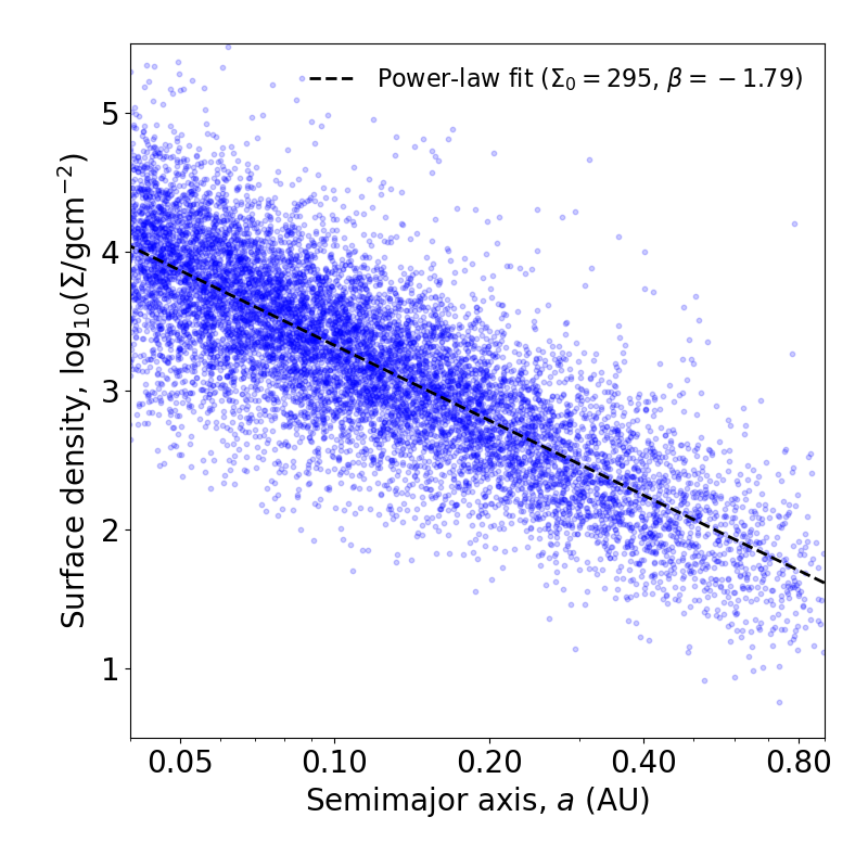
MMEN of a simulated observed catalog — The solid surface densities and MMEN fit to a simulated observed catalog.

Note

In this example, the function solid_surface_density_CL2013_given_observed_catalog takes the observed catalog, uses a mass-radius relation to draw a set of planet masses from the planet radii, and enforces a limit on the maximum mass via max_core_mass before calling the function solid_surface_density_CL2013 we started with at the top of this page.

We’ve removed the maximum core mass limit (by setting max_core_mass=np.inf) to show you the broad range of surface densities arising from the broad range of planet masses. By default, it is set to 10 Earth masses.